Note: I have blind spots. With limited formal training in advanced statistics, often I won’t know what I don’t know. One key reason to start this blog was to iron out those blind-spots, and all help in that regard is welcome.
Introduction
I look at hypothesis testing in three stages:
Null view of the world.
Alternate view of the world.
Uncertain but observable underlying reality.
My previous post created a bit of kerfuffle around whether or not there is an implicit assumption that the Type 1 Error Rate is 50% when applying a decision rule that compares the simulations of two distributions under differing parameters.
Is \(H_0 : p_b = p_a\) same as \(H_0 : |p_b - p_a|=0\) ?
When do we commit a Type 1 Error? In the simplest terms, when planning an experiment, I have to define a rejection region where I will reject the null hypothesis. When the observed reality appears in the rejection region, there is a chance that it was a fluke and the there is no underlying causal effect.
It can also be the case that the underlying effect is real and in fact larger or just at the boundary of the rejection region. Either way rejecting the null was the right decision but I cannot really know. There will always be a chance that even with a large enough effect there really is no difference between the two samples being compared.
When I observe the data, I either reject the null or I don’t (or say that there isn’t enough evidence to apply the decision rule). It’s not possible to know if I committed an error or if I correctly rejected the null. We hope to minimise the probability of making an error in the planning stage, but after collecting the data the decision is made and that is that.
The purpose of this section is to point out how expressing the null hypothesis as \(H_0 : p_b = p_a\) while being technically correct, can be misleading. It makes it seem like we are comparing two different random variables, both of which are ultimately an estimator of the unobservable (mean?) conversion rate of individual Bernoulli trials under two different treatments. But really all we do is either take their ratio or difference and study that. The ratio or the difference is a different random variable and studying that variable in a hypothesis test is not the same as estimating the conversion rates of two designs.
When are two random variables equal (or almost equal)? Let’s take the less strict definition, that when they are ‘equal in distribution’. That is, they have the same set of possible values and the same probabilities for all of those values.
Even an A/A test does not result in a situation where the estimates of \(p_a\) and \(p_b\) would be exactly equal. Essentially this null hypothesis, if applied strictly, would result in a situation where an effect is always present.
In practice, if we force ourselves to not use the difference of estimated rates as the test statistic, we can choose to simulate data from two distributions and count the number of times one exceeds the other. Let’s understand this with a code exercise. We’ll use the following values for the planning stage:
Historical Rate: 10%, MDE: 5%, T1 Error Rate = 10%, Power = 90%, Type = 2-tailed
We’ll also run a hypothetical A/B test where the observed lift was 2.2%. For simplicity, we assume that the observed rate for design A was 10%. Note that this is the observed reality, and we are always uncertain about it.
Show the code
library(tidyverse)library(glue)library(furrr)library(ggthemes)library(progressr)library(extrafont) #You can skip it if you like, it's for text on charts.library(knitr)##Modify this as per your computing setupplan(strategy ='multisession',workers =16)
Critical lift boundaries(%) for selected parameters under null view that 𝛿=0: -2.810%, 2.810%
Now let’s apply the test of proportions for the hypothetical A/B Test.
Show the code
obs_lift=.022x<-prop.test(x =c(p1,p1*(1+obs_lift))*n, n =c(n,n))x
    2-sample test for equality of proportions with continuity correction

data:  c(p1, p1 * (1 + obs_lift)) * n out of c(n, n)
X-squared = 1.6541, df = 1, p-value = 0.1984
alternative hypothesis: two.sided
95 percent confidence interval:
 -0.00554429  0.00114429
sample estimates:
prop 1 prop 2
0.1000 0.1022
We see that the p.value of 19.84% is above the p.value threhsold of 10% when the observed positive lift 2.2% is within the critical lift boundaries for our 2-tailed test of proportions.
Now let’s use a simulation to analyse the same hypothetical experiment.
Show the code
#Simulations for the same boundarypp2 = p1*(1+obs_lift)qq2=1-pp2n_sim =10^6set.seed(132)sim_p1 =rnorm(n=n_sim, mean=p1,sd =sqrt(p1*q1/n))sim_p2 =rnorm(n=n_sim, mean=pp2,sd =sqrt(pp2*qq2/n))pct_superior = (sum(sim_p2>sim_p1))/n_sim
When estimated E(pa) = 10% and E(pb) = 10.22%, the simulated values of pb exceed pa 90.26% of the time.
If we interpret this to be the same as p.value, then the p.value here is ~9.74%, which is below the threshold of 0.1%. But how can that be?
The answer lies in the fact that the two comparisons are not the same. The latter comparison is one tailed. For continuous variables, if I were to sum \(p(p_a>p_b)\) and \(p(p_a<p_b)\), this would sum to 1. This is like saying that an effect is always present.
Let’s break character a bit and use the ratio of the two simulations, and look at the quantiles.
Quantiles of the ratio of conversion rates from design B and design A’s simulated data:
Percentage of simulations where ratio is at or below 1: 9.74%.
Notice how the 5th percentile of the ratio of the two simulations is below 1. This is important. Now let’s assume that observed lift of our hypothetical experiment was in fact 2.81%, which is at the boundary of our rejection region under the null defined as 𝛿=0 under the 2-sample test of proportions. At lift = 2.81%, the null will be rejected in favour of design B by the 2-sample test of proportions.
Let’s simulate this scenario.
Show the code
#Simulations for the same boundarypp2 = p1*1.0281qq2=1-pp2n_sim =10^6set.seed(132)sim_p1 =rnorm(n=n_sim, mean=p1,sd =sqrt(p1*q1/n))sim_p2 =rnorm(n=n_sim, mean=pp2,sd =sqrt(pp2*qq2/n))
Quantiles of the ratio of conversion rates from design B and design A’s simulated data:
Percentage of simulations where ratio is at or below 1: 4.89%
At the boundary condition, the 5th percentile of the ratio of the conversion rates is above 1.
If the decision rule is changed,
From: checking if the count of the ratio exceeds 1 at least (1-𝛂)% of times
To: checking that the 𝛂/2 percentile value of the simulation ratios is above 1,
the two decision criteria are essentially at par. But this is to be expected. 5th Percentile is α/2 for our chosen value of α=10%. There is only a 4.8% chance that true conversion rate of design B is worse than that of design A.
Ergo, we are insisting on both a two-tailed comparison and defining a zone of uncertainty by looking at the 5th percentile of the ratio of the two simulations. Please note that if \(\hat{p_2}<\hat{p_1}\), the comparison needs to be performed for the inverse ratio (you can add them if you prefer, thereby making the comparison direction agnostic).
In conclusion, the two definitions of the null hypothesis are indeed equivalent but in practice the latter can lead to improper application.
Gripe with the ECDF decisioning rule used in Bayesian A/B Testing
This is my gripe with the application of ecdf in this article on Bayesian A/B testing. It’s not that it is incorrect, but that people often misinterpret this decisioning rule and end up applying a 1-tailed test while insisting that the IBE model leads to reduction in sample-size requirements as compared to a 2-tailed test of proportions.
If we stick to using the decisioning rule that the ECDF at 1 for the ratio of conversion rates should be less than the p-value threshold (or its half for a 2-tailed test), the decision rule will work at par in an IBE Bayesian framework with an uninformative Beta(1,1) prior.
This should hopefully become more apparent in the next section.
Another minor gripe is claiming that you get an entire range of values for the possible improvement using an ECDF. While this is technically correct, a confidence interval around the mean observed lift also provides an entire range of possible values, even though there are subtle differences in the interpretation of the two results.
Most business executives and product people I worked with took me to the cleaners at the mention of a confidence (or credible) interval. It’s incredible how little confidence they had in me.
Practically, we are almost always focused on the mean or median value.
Why I am of the opinion that defining \(H_0 : p_b = p_a\) leads to an inflated T1 Error Rate?
I am open to being criticized here and in fact I have debated this with myself many times. I figured that the only way to know is to spark a public fallout, so here goes nothing.
The premise is that the error is in the application, not the mathematical equivalence of the two formats of expressing the null hypothesis.
Let’s look at a very practical example: the A/A test. If I run an A/A for a sufficient duration, do I expect to reject the null half the time or 𝛂% of the time or all of the time?
The purpose of an A/A test is to detect anomalies in your experimentation infrastructure. A signal that there is a difference in conversion rates observed in two samples indicates potential issues with the setup or infrastructure implementation.
In a frequentist perspective, just about any difference is detectable given you collect enough data. And it’s almost never the case that the difference of two samples of conversion rates will be zero.
But let’s assume that we plan it like a usual fixed-sample test. We’ll use a historical rate of 10%, an MDE of 5%, 𝛂 of 20% and power of 90%.
We’ll simulate 10^6 A/A tests of sample-size ‘n’. We’ll reject the null hypothesis in four ways: once with a test of proportions, once with comparing \(p_a\) and \(p_b\) in simulations - both one tailed and two tailed, and once by comparing them at a threshold.
The table below indicates the number of times (% of simulations) we reject the null in favour of either A1 or A2:
Show the code
kable(dt0, digits =2)
null_rejected
direction
pct
FALSE
NA
80.4
TRUE
A1>A2
9.8
TRUE
A2>A1
9.8
Probability of rejecting the null with a two tailed test of proportions per table above: 19.6%.
Probability of rejecting the null with a one tailed comparison at zero threshold (x1 above): 49.96%.
Probability of rejecting the null with a two tailed comparison at zero threshold (x2 above): 100%.
Probability of rejecting the null with a two tailed comparison at critical lift threshold (x3 above): 19.49%.
Of course it’s trivial to claim that if the boundary condition is at ‘any difference’ goes, the null will be rejected 50% of the time for a one-tailed comparison and 100% of the time for a 2-tailed comparison.
What’s interesting however is that if I apply the same critical boundary as the proportions test to the simulations, my rate of rejecting the null was more or less the same (prob 1 and 4 above).
If I define no zone of uncertainty, I cannot really run an A/A test. We are ALWAYS comparing either the ratio or a difference in rates irrespective of whether we use a parametric test or a simulation. So why express the null as \(H_0 : p_b = p_a\) and cause confusion?
This is another reason why I am skeptical of the decision-system whereby we simply compare the instance of the simulations under \(p_b\) that are greater than those under \(p_a\). This system does not seem to work very well unless I always use a 1-sided comparison. In an unqualified 2-sided comparison, a simulation tells us that either A1 or A2 is always better, since the two rates are never exactly equal.
What about an IBE Bayesian A/A Test?
It’s simple, really. We take “N” draws from both posterior simulations and then create a ratio as A2/A1 in the usual way. To keep the comparison same as a 2-tailed 2-sample test of proportions, we use the following decision rule: \(p(ECDF(ratio <= 1)) < p.value\ threshold/2\).
Yes, this is no rocket science. But my blog isn’t aimed at seasoned stats professionals/academicians but rather at a more general audience, to who all of this may not be immediately obvious.
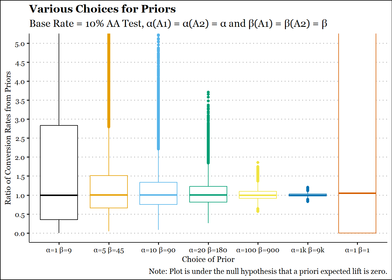
The key however is defining a prior. There is no real point in using a Bayesian methodology if stronger assumptions aren’t made, so we won’t be using an uninformative prior like Beta(1,1). And since we are planning an A/A test, we will be keeping the parameters equal, i.e. 𝛂A1 = 𝛂A2 = 𝛂 and 𝛃A1 = 𝛃A2 = 𝛃.
We kept our historical rate as 10%, so really, the question is whether the prior should be beta(10,90) or beta(1000,9000).
Show the code
p1 = .1prior_alpha =c(10,50,100,200,1000,10000,1)*p1prior_beta =c(10,50,100,200,1000,10000,1)*(1-p1)n_sim =10^5set.seed(145)prior_ratios =pmap(list(.x = prior_alpha,.y = prior_beta, nn =n_sim),.f = \(.x,.y,nn) rbeta(nn,.x,.y)/rbeta(nn,.x,.y)) |>bind_cols() |>rename_with(.fn =~LETTERS[1:7]) |>pivot_longer(cols =everything(),names_to ='Priors',values_to ='Ratio') |>mutate(Priors =factor(Priors,ordered = T))ggplot(prior_ratios,aes(y = Ratio,x=Priors, col = Priors)) +geom_boxplot() +coord_cartesian(ylim =c(0, 5)) +labs(title ="Various Choices for Priors",subtitle ="Base Rate = 10% AA Test, \u03B1(A1) = \u03B1(A2) = \u03B1 and \u03B2(A1) = \u03B2(A2) = \u03B2",caption ="Note: Plot is under the null hypothesis that a priori expected lift is zero.",x ="Choice of Prior",y ="Ratio of Conversion Rates from Priors",parse = T) +scale_x_discrete(labels =paste0("\u03B1=",c("1","5","10","20","100","1k","1")," \u03B2=",c("9","45","90","180","900","9k","1"))) +scale_y_continuous(breaks =seq(0,5,.5), minor_breaks =seq(.25, 4.75,.5)) +scale_color_colorblind() +theme_clean() +theme(text=element_text(family="Georgia"), legend.position='none')
The choice of beta(10,90) seems reasonable. It doesn’t concentrate too heavily around a ratio of 1 and is more or less symmetric about 1. You can already see that the distributions can be right-skewed. Of course you could resolve that by using a difference instead of a ratio. But a ratio seems to be used more often by practitioners and proponents. The outcome of a beta(1,1) is also plotted for comparison. Clearly the range is too vast and it has no meaningful use.
Now let’s perform 10^4 A/A tests (lower count as we also need to simulate the posterior every time). But now comes the key question. In the frequentist paradigm, we just sampled from a normal distribution and each draw of \(\hat{p}\) was an A/A test.
In the Bayesian paradigm, we are really dealing with the probability of an event. So, do we draw from the normal distribution or something else entirely? What we know is that the average rate has to be 10% and that we will collect same ‘n’ data-points as earlier. Since we kept ‘n’ constant earlier, we can continue to do the same. In fact, we had already assumed that our underlying data is binomially distributed - this is what allows our posterior to be beta distribution (read: conjugate priors).
The table below indicates the number of times (% of simulations) we reject the null in favour of either A1 or A2:
Show the code
kable(dt1, digits =2)
Comparison
Nulls Rejected(%)
A2>A1
10.20
A1>A2
10.09
Our rate of rejecting the null was slightly higher than 20%.
This is despite the fact that using the same prior for both \(p_{A1}\) and \(p_{A2}\) should lower it as we are adding a priori evidence for the baseline being the same. In all honesty this is more or less a simulation artifact and we can use a stronger prior like beta(100,900). But the gaps in the beta-binomial approach should now be clear.
IBE Bayesian A/A Test - Conclusions
Notice how we consciously made a comparison on both sides (A2>A1 and A1>A2). When running an A/B test, we typically are looking to implement a new design – there is a built-in directional bias. This gets reflected in the implementation when typically the ratio is compared on only one side for an A/B test. But an A/A test forces us to rethink this. Clearly the comparison should be made on both sides.
Before any data is collected, it is equally likely that design B is worse than design A. Yet, this isn’t taken into account when practitioners compare the ECDF of ratio of conversion rates solely in the direction where B is greater.
In practice, I have seen practitioners first check the direction, and then take the ratio as \(p_{b}/p_{a}\) or \(p_{a}/p_{b}\), whatever is convenient. It should be obvious that this is a post-hoc selection of direction, and obviously unless the p-value is halved, this is also equivalent to a 1-tailed test.
Once again, the problem isn’t the math, the problem is in the implementation. There are clear disadvantages to the IBE model.
…
We examined some critical issues in implementation errors when we express our null hypothesis in frequentist approach as: \(H_0: p_b = p_a\).
We also examined some critical issues in the implementation of Bayesian tests that utilise the IBE model. We also saw that priors on conversion rate ratio can be skewed.
I want to reiterate that the fault is in the model and the implementation, not Bayesian A/B (or A/A) testing. There are more tractable ways of running Bayesian experiments which we will explore in future posts.