Technically Correct Bayesian A/B Testing without Monte Carlo Simulations
Why estimating conversion rates is not the same as running an A/B Test
We use a simple and tractable mathematical model that can be solved algaebrically. We demonstrate one key omission in the IBE approach: that of the alternative hypothesis. We also look at a sample-size imputation method to help with the process of building priors.
Note: This is part 3 of a series on Bayesian A/B testing.Part 1 discusses the most common approach and its limitations. Part 2 uses simulations of A/A tests to delve deeper.
Introduction
In the previous posts we explored the the limits and problems in implementation of the Independent Beta Estimator(IBE) approach of Bayesian A/B Testing.
As a recap, there are following modeled and implementation errors in an IBE Bayesian test:
Poor choice of priors - too strong, too useless, or improperly estimated,
Inadvertently running a 1-tailed test while believing you are running a 2-tailed test,
Implicit definition of a non-rejection region for the observed lift by comparing ratios or differences rather than an explicit prior on the MDE/modeled lift itself.
Implicit definition of a common prior on the baseline conversion rate for the two designs rather than having the model explicitly use a common prior for the lift (e.g. \(lift \sim N(0,.2)\))
Today we’ll discuss an alternative approach that uses a prior directly on the expectation around lift. I first came across this approach in Eppo’s reference documentation1 on their statistical engine. While my preferred model is the Logistic Transformation Model (Hoffmann, Hofman, and Wagenmakers 2022), I will be discussing this Normal-Normal (both prior and posterior are normally distributed) approach first for a few key reasons:
Right off the bat the mathematical model reflects what we are trying to do: establish a conversion rate difference between two designs, i.e., lift rather than model two independent conversion rates, followed by forcing a common prior, and then bringing in the modeling of lift through the backdoor.
The model also explicitly honours the idea that the difference in rates cannot vary wildly beyond a certain range under most circumstances.
It’s an elegant model in the sense that prior and the posterior are both normally distributed. Further, just like the IBE model, the posterior can be arrived at analytically. While in both models there really is no need to simulate the posterior distribution of the lift as both can be solved analytically, the normal-normal model on the (possible values of) lift makes it obvious. This is because there is no requirement of taking the ratio or difference of two independent estimators.
Let’s become Normal-Normal: The model
There is nothing complicated to it. The prior is considered to be normally distributed with the parameters set to some initializing values. Please note that in this illustration the prior is on the difference between conversion rates \(\hat{p}_b - \hat{p}_a\) and not relative difference, i.e. lift. You can think of it as akin to a prior expectation about the average treatment effect.
The likelihood is also considered to be normally distributed, i.e., there is a single observation of the lift after ‘N’ data points are collected and the difference in conversion rates is modeled as normally distributed. You can also imagine it as multiple Bayesian updates after collecting some ‘n’ data-points at some regular or irregular intervals. Under usual assumptions of the Classical CLT, this observed difference in conversion rates (i.e. the estimated ATE) of two designs can also be considered to be normally distributed. This leads to a posterior difference in rates, \(\hat{\Delta}_{post}\) , with parameters described as:
For a formal derivation of how to arrive at the Normal-Normal posterior, please refer this document.
Note that their is a minor dissonance in this model. For most A/B tests, our observations are after-all event counts – a user takes or doesn’t take an action of interest, as a function of the design they saw (i.e. CRO). Thus, the model is not truly representative of the data generating process when modeling event rates or proportions. This is the primary reason for my preference of the Logistic Transformation Model (LTT) for proportions or CRO.
But the ability to run an analysis quickly with just plug-and-play values is useful and most often the results won’t be particularly different. Therefore, this model works great for a quick sense-check as well as for planning and scenario analysis before running an experiment.
We’ll now look at the process of defining the parameters for the prior.
Defining the Prior
Prior under the Null Hypothesis \(\mathcal{H}_0:\Delta = 0\)
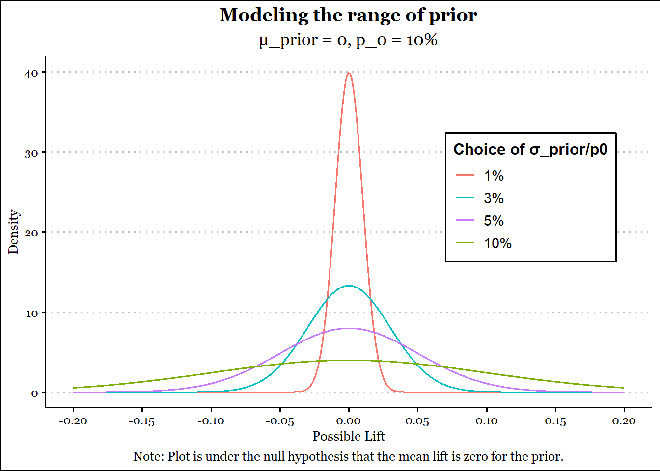
Of course, under the null, \(\mu_{prior} = 0\). All we need now is an appropriate value for \(\sigma_{prior}\). For convenience, we’ll be using standard deviation instead of the variance. \(\sigma_{prior}\) sets our a priori expectation for the range over which difference in rates can vary. We can use a wide range like \(\sigma_{prior} = .05\) or a narrow range like \(\sigma_{prior} = .01\).
Typically, however, in A/B testing we do the analysis in terms of the lift and a base or historical rate. Therefore, we can define \(\Delta_{prior}/p_{0} = \mathcal{l}\) where \(\mathcal{l}\) is a choice of lift and \(p_{0}\) is the historical conversion rate. Thus, we are defining the range relative to the base rate.
Please note that Eppo’s reference model is based directly on \(\mathcal{l}\).
Let’s use \(p_{0} = 10\%\) and model various values of plausible (not observed) range of lift2, viz. 1%, 3%, 5% and 10%. Please note that we are plotting the null for mean lift of 0. The gymnastics above are to visualise the impact of \(σ_{prior}/p_{0}\).
Show the code
library(tidyverse)library(glue)library(furrr)library(ggthemes)library(progressr)library(extrafont) #You can skip it if you like, it's for text on charts.library(gridExtra)library(knitr)library(rlang)##Modify this as per your computing setupplan(strategy ='multisession',workers =16)
Show the code
p0 = .1lift =c(.01,.03,.05,.1)chart_labs =glue("{lift*100}%")mu_p =0sig_p = p0*lift# We are plotting lift instead of difference, but we can plot difference by changing lift[] to sig_p[]. It's just scaling.paste0("ggplot() + ",glue_collapse(glue("geom_function(fun = dnorm, n =10^4, args=list(mean=mu_p,sd=lift[{i}]), aes(col = chart_labs[{i}]),lwd=.6)", i =seq_along(lift)),sep =" + ")) -> cceval(parse(text = cc)) +scale_color_discrete(breaks=chart_labs) +scale_x_continuous(limits =c(-.2,.2), n.breaks =11) +labs(title ="Modeling the range of prior",subtitle ="\u03BC_prior = 0, p_0 = 10%",caption ="Note: Plot is under the null hypothesis that the mean lift is zero for the prior.",color ="Choice of \u03C3_prior/p0",y ="Density",x ="Possible Lift",parse = T) +theme_clean() +theme(text=element_text(family="Georgia"), legend.text.position='right', legend.position =c(.8,.6),plot.caption =element_text(hjust =0.5),plot.title =element_text(hjust =0.5),plot.subtitle =element_text(hjust =0.5))
Figure 1: Modeled Priors
No surprises here. A larger value for σprior (possible lift) leads to a larger range over which the prior is spread out about 0. Essentially, a larger value indicates more uncertainty about zero and a smaller value indicates less uncertainty about zero. Since the prior is set to a mean value of zero, a smaller value for σprior indicates both a stronger and a more conservative prior. You can also see that the prior is symmetric about zero. Most of the time this is a good thing.
Generally speaking, as the baseline rate gets larger, the observed lifts during an experiment will be smaller, while also being meaningful. This is to say that a 1% relative improvment on 70% is comparable to a 5% relative improvement on 10%. Ergo, an absolute value like \(\sigma_{prior}=0.01\) may work well across most circumstances.
Strength of Prior – Assessment through imputed sample-size
When usually running A/B tests for conversion rate optimisation, we generally tend to understand that the more data we collect, the less uncertainty we have about our estimate of the lift (or of individual designs’ conversion rates for that matter).
In my opinion, we can extend that analogy to the Normal prior as defined in Equation 1 to impute a sample-size. This helps us understand how strong the prior is as a function of the amount of data we hope to collect. Alternatively, we can use this figure to plan the amount of data we will collect for an A/B test. Please note that strictly speaking these are not Bayesian concepts, or even established academic concepts of any sort.
But in my opinion even a Bayesian inference framework should have some underpinnings on the amount of data we should reasonably collect before arriving at a decision. And this method helps us take an educated guess in that direction.
Essentially, all we do is assume that we arrived at the range of our prior by collecting some data about a design and we ran an A/A test for that design. In this case, we can safely say that \(\mu_{prior} = 0\) and \(\sigma_{prior} = \sqrt{\frac{p_0.q_0}{\mathcal{n}} + \frac{p_0.q_0}{\mathcal{n}}}\), where \(p_0\) becomes the conversion rate for this hypothetical A/A test (\(q_0 = 1-p_0\)).3
For a given choice of \(\sigma_{prior}\), we can invert this value to arrive at \(\mathcal{n}\). Let’s try this for \(p_0 = 12\%\) .
Table 1: Imputed Sample size of the Prior (p0 = 12%)
Lift
σ_prior
Imputed SS
1%
0.0012
146,667
3%
0.0036
16,297
5%
0.0060
5,867
10%
0.0120
1,467
Clearly a narrower prior indicates a larger imputed sample-size. The only question that remains is, “how do we use this?? Well, my suggestion is to collect at least as much data as the imputed sample-size of the prior. And perhaps not use priors that are too narrow if the amount of data that can be reasonably collected does not match-up.
I will readily admit that the choice of prior is not a straightforward thing. To be fair, it’s equally convoluted in the IBE methodology – it’s just hidden way from the user through uninformative priors in some mainstream stats engines. I will cover the topic of selecting priors in a separate post.
For programs that have a long history of experimentation, it should be possible to rely on historical results around observed lifts for similar experiments or for experiments where the conversion rate was similar to what is expected in the upcoming experiment.
Running a truly Bayesian Hypothesis Test
Where is the (point) alternative hypothesis?
The astute reader would have noticed that in our previous discussions around Bayesian A/B and A/A Testing (Part 1 and Part 2 respectively), we never really defined a point alternative hypothesis, i.e., an MDE, like we do in frequentist A/B testing.
In the frequentist test of proportions, defining a power (and therefore a sample-size that controls both Type 1 and Type 2 errors), requires defining the alternative at a point, i.e. it demands an effect-size or MDE. (\(\mathcal{H}_a: \Delta = \big\lvert p_0.MDE \big\rvert\))4.
So far we have not defined an alternative hypothesis, let alone an alternative around an MDE. This is where Bayes Factor comes in. The good news is that for our specific use-case, we don’t require the definition of an MDE, as we are not really defining a formal sample-size requirement5.
We can therefore continue with defining our alternative hypothesis in the usual way as a two-sided non-zero comparison. This brings us to the Bayes Factor.
Bayes Factor
I first came across this concept in Will Kurt’s blog6.
Bayes Factor is essentially a ratio of relative evidence favouring one modeling assumption over the other, or one hypothesis over the other.
Formally, let \(\mathcal{M}_i\) denote possible models for explaining data \(\mathbb{\mathcal{y}}\), where \(\mathcal{i} \in [1,2]\)7. Then,
where the first term is the posterior odds and the second term is the inverse of prior odds. Bayes Factor is therefore the ratio of likelihood of the observed data under two different modeling assumptions. In our case this simplifies to the null and the alternative hypothesis respectively.
Please note that this ratio is invertible, i.e. \(\mathcal{BF}_{12} = 1/\mathcal{BF}_{21}\). Also note that in most circumstances both (or all) models are a priori considered equally likely, i.e., the prior odds are 1. The Bayes Factor then reduces to the ratio of the posteriors under the two models or hypotheses.
For a more detailed explanation of this section and the next one, I refer you to this excellent paper.
Table 2: The Bayes factor scale as proposed by Jeffreys (1998).
\(\mathcal{BF}_{12}\)
Interpretation
>100
Extreme evidence for \(\mathcal{M}_1\)
30−100
Very strong evidence for \(\mathcal{M}_1\)
10−30
Strong evidence for \(\mathcal{M}_1\)
3−10
Moderate evidence for \(\mathcal{M}_1\)
1−3
Anecdotal evidence for \(\mathcal{M}_1\)
1
No evidence
11−13
Anecdotal evidence for \(\mathcal{M}_2\)
13−110
Moderate evidence for \(\mathcal{M}_2\)
110−130
Strong evidence for \(\mathcal{M}_2\)
130−1100
Very strong evidence for \(\mathcal{M}_2\)
<1100
Extreme evidence for \(\mathcal{M}_2\)
With most of the math out of the way, we can finally tackle the last remaining piece: the Savage-Dickey Density Ratio.
Comparing Densities at a point null using the Savage-Dickey Density Ratio
In our usual hypothesis testing framework, we express our two models as:
where \(\mu\) represents the difference in conversion rates in terms of the notation we have used so far.
Ergo, \(\mathcal{M}_1 = \mathcal{H}_0\) and \(\mathcal{M}_2 = \mathcal{H}_1\).
The Savage-Dickey Density ratio simplifies the computation of the Bayes Factor \(\mathcal{BF}_{01}\) to the ratio of density of the prior at the point null to that of the density of the posterior at that null.
Consider two competing models on data \(\mathbb{y}\) containing parameters δ and φ, namely ℋ0: δ = δ0, φ and ℋ1 : δ, φ. In this context, we say that δ is a parameter of interest, φ is a nuisance parameter (i.e., common to all models), and ℋ0 is a sharp point hypothesis nested within ℋ1. Suppose further that the prior for the nuisance parameter φ in ℋ0 is equal to the prior for φ in ℋ1 after conditioning on the restriction – that is, p(φ | ℋ0) = p(φ | δ = δ0, ℋ1). Then:
For a proof you can look at the citation above or check this link here.
In the context of our models and assumptions, \(\delta = \mu_{post} = 0\), and \(\varphi = \sigma_{post}\) is the nuisance parameter. It’s trivial to show that without data \(\mathbb{y}\), \(\mu\) and \(\sigma\) reduce to their values from the prior.
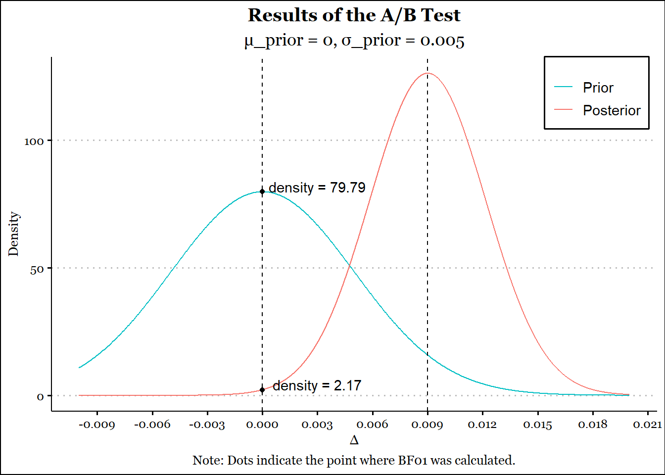
Thus, in order to calculate \(\mathcal{BF}_{01}\), all we need is the densities at \(\delta = 0\) for the posterior and the prior. Let’s try an example.
Run the A/B test already!
We’ll run an A/B test for 12K users for both designs, and let’s say the conversion rates were 10.5% and 12% for A and B respectively. Our prior is set to parameters \(\mu_{prior} = 0;\; \sigma_{prior} = .005\). We are assuming that \(\sigma\) was derived from a base rate of 10% and a usual lift range of 5%.
chart_labs =c("Prior", "Posterior")ggplot() +geom_function(fun = dnorm, n =10^3, args=list(mean=mu_pr,sd=p0*lift), aes(col = chart_labs[1])) +geom_function(fun = dnorm, n =10^4, args=list(mean=mu_po,sd=sqrt(var_po)), aes(col = chart_labs[2])) +geom_point(aes(x=0,y=dens_pr)) +annotate("text", x = .003, y = dens_pr+2, label =glue("density = {round(dens_pr,2)}")) +geom_point(aes(x=0,y=dens_po)) +annotate("text", x = .003, y = dens_po+2, label =glue("density = {round(dens_po,2)}")) +geom_vline(xintercept =0,linetype =2) +geom_vline(xintercept = mu_po,linetype =2) +scale_color_discrete(breaks=chart_labs) +scale_x_continuous(limits =c(-.01,.02), n.breaks =11) +labs(title ="Results of the A/B Test",subtitle =glue("\u03BC_prior = 0, \u03C3_prior = {y}",y = p0*lift),caption ="Note: Dots indicate the point where BF01 was calculated.",color =element_blank(),y ="Density",x ="\u0394",parse = T) +theme_clean() +theme(text=element_text(family="Georgia"), legend.text.position='right', legend.position =c(.9,.9),plot.caption =element_text(hjust =0.5),plot.title =element_text(hjust =0.5),plot.subtitle =element_text(hjust =0.5))
Figure 2: A/B Test Results
In this particular case, the prior adequately regularized the collected data, which we can see from the reduced lift (8.58% as opposed to 14.29%).
There is about 97.35% probability in favour of \(\mathcal{H}_1\).
A caveat here: if we were to run a frequentist 2-sample test of proportions in this scenario, the power for the comparison (\(\alpha=10\%\), \(p_0=10.5\%\) and \(m.d.e.=10\%\)) would be around 83%. For the amount of data we have collected, we could have just as easily run a frequentist A/B test, for all practical purposes. (An observed lift of 8.5% would be detectable in this scenario with appropriate error controls).
This is to be expected as a prior defined about 0 is naturally going to reduce an observed lift, depending on its relative strength to the data collected.
Using the Ratio instead of difference
For comparison’s sake, let’s run the same scenario as above but with relative difference defined as \(\frac{\hat{p_b}}{\hat{p_a}}-1\), as opposed to the absolute difference. The distribution of the above statistic is also considered to be Normal albeit under some approximations to arrive at the \(\hat{\mu}_\Delta\) and \(\hat{\sigma}_\Delta\) via Taylor’s expansion (Duris et al. 2018) or the delta method.
Table 4: Outputs from the ratio based A/B Test (S.S. are per design).
Attribute
Value
Observed lift
14.29%
Posterior Lift
8.45%
\(\mathcal{BF}_{01}\)
0.0474
\(\mathcal{BF}_{10}\)
21.11
Imputed S.S. (Prior)
7,200
Imputed S.S. (Post.)
20,285
p(\(\mathcal{H}_1\))
95.48%
Advantages of the Bayesian Framework
As is obvious, just about any framework will work if you can collect enough data.
The value of the Bayesian framework is therefore not in economising the sample size, although that can be a use-case in certain scenarios. Rather it’s value is in:
The regularizing of the observed data through a well-defined prior.
Allowing you to define a prior using historical experiments.
Direct interpretability: instead of butting our heads about a mythical p-value, we get a straightforward interpretation through a Bayes Factor (odds in favour of a hypothesis) and the probabilistic evidence in favour of a hypothesis of interest.
The posterior distribution is exactly what you think it is: a range of possible lifts with some values being more probable than others.
Combined with an appropriate revenue function, this allows you to calculate the expected revenue over a full range of possibilities.
As we go along and explore more complex models, we’ll see that we can also adjust the prior odds of the model. This may be useful if let’s say we are running a series of experiments and we already have some evidence in favour of the alternative hypothesis from previous experiments.
No peeking adjustment required (usually): Since today’s posterior is tomorrow’s prior, adjustments are not required for checking results at the interim intervals. I am not completely sure about this but there seems to be some consensus around this.
Caveats of the Normal-Normal Model
The core advantage of this approach is of course being able to use it without needing to run simulations of any sort. There are however certain caveats that should be highlighted:
Not the most accurate model: At the end of the day, the point of Bayesian Inference is to define your model as closely as possible to the data generating process9. The utility of the IBE model comes precisely from resembling the actual process of observing a series of conversion events.
The model places some non-zero weight on differences that cannot occur. The difference of two rates cannot exceed the limits of -1 and 1. This is one of the reasons why this model is not as accurate as say a well defined Hierarchical Bayesian Model like the Logistic Transformation Model of A/B Testing (Wagenmakers et al. (2010)). Of course we can rely on the ratio metric to address this.
The prior and the posterior will always be symmetric about the mean. While this is a desirable property most of the time, sometimes it might be better to have a skewed or a heavier tailed distribution. Even if we were to change just the prior to a more appropriate distribution, the parametric simplicity due to it being the conjugate of the posterior would very often disappear. Then we are back to simulations.
Despite all the caveats, I have used this approach extensively as a first pass due to its simplicity. The eventual result may come from a more complex model, but this should definitely be the multi-utility tool in your A/B testing kit.
And hey, most of the time the complexity may not be required, so why not save on the electricity needed to run those MCMC simulations?
…
We looked at the Normal-Normal model of running a Bayesian A/B test. We combined it with the Savage-Dickey Density Ratio to run a bi-directional superiority (inferiority) hypothesis test for a point null defined on a parameter of interest.
Please note that there are version of this approach that can handle equivalence/non-inferiority testing as well as directional superiority (inferiority) hypothesis testing.
We explored ways in which the above approach is an upgrade over the IBE model of Bayesian A/B testing.
References
Duris, Frantisek, Juraj Gazdarica, Iveta Gazdaricova, Lucia Strieskova, Jaroslav Budis, Jan Turna, and Tomas Szemes. 2018. “Mean and Variance of Ratios of Proportions from Categories of a Multinomial Distribution.”Journal of Statistical Distributions and Applications 5 (1). https://doi.org/10.1186/s40488-018-0083-x.
Faulkenberry, Thomas J. 2019. “A Tutorial on Generalizing the Default Bayesian t-Test via Posterior Sampling and Encompassing Priors.”Communications for Statistical Applications and Methods 26 (2): 217–38. https://doi.org/10.29220/csam.2019.26.2.217.
Hoffmann, Tabea, Abe Hofman, and Eric-Jan Wagenmakers. 2022. “Bayesian Tests of Two Proportions: A Tutorial with r and JASP.”Methodology 18 (4): 239–77. https://doi.org/10.5964/meth.9263.
Wagenmakers, Eric-Jan, Tom Lodewyckx, Himanshu Kuriyal, and Raoul Grasman. 2010. “Bayesian Hypothesis Testing for Psychologists: A Tutorial on the SavageDickey Method.”Cognitive Psychology 60 (3): 158–89. https://doi.org/10.1016/j.cogpsych.2009.12.001.
Footnotes
Eppo’s model is based on lift or relative difference. I am using the difference in rates or absolute difference.↩︎
I am intentionally avoiding calling the plausible lift ‘MDE’ as that would be misleading.↩︎
Or we can define an MDE and use \(\sigma_{prior} = \sqrt{\frac{p_1.q_1}{\mathcal{n}} + \frac{p_2.q_2}{\mathcal{n}}}\) where \(p_2 = p1.(1+MDE)\).↩︎
I understand that there will be disagreements here, but I request the seasoned academician to let this one slide for now.↩︎
I believe it’s possible to define the power of a Bayesian Hypothesis Test using a Bayes Factor, but that’s something I’ll cover in a separate post.↩︎
I owe my initiation into Bayesian statistics to this blog. You could say that my own blog is inspired from Will Kurt’s work.↩︎
We can have more than two models, but right now we are constraining ourselves to two, the null and the alternative hypothesis.↩︎
Since the Bayes Factor in our case is essentially odds in favour or against any one of the two hypothesis, we can convert the odds to a probability.↩︎
This gets into the cogency v/s similitude debate, whereby we decide what’s more important - a complex process that is closer to the DGP v/s a simpler process that gives a very close approximation. Thank you Tyler Buffington for pointing this out.↩︎