Running a classical Bayesian A/A Test, and paying for our priors.
A discussion on the fault in our Bayesian Stars through an A/A Test
We look at how an A/A test seems to reveal some common flaws in implementation of the IBE Bayesian model. We also look at some poor decisions made at the time of selecting a prior in A/B Tests.
Note: This is part 2 of a series on Bayesian A/B testing. Check part 1 here.
Introduction
There’s nothing better than an A/A test to bring all your weird modeling assumptions to the table, because it takes one key challenge away - that of detecting a true difference between designs.
We explore the the limits and problems in implementation of the Incremental Beta Estimator(IBE) approach of Bayesian A/B Testing.
For a discussion on what the model is, check part 1 of this series.
Note: The first section is a reproduction from here.
As a recap, there are following modeled and implementation errors in an IBE Bayesian test:
Poor choice of priors - too strong, too useless, or improperly estimated,
Inadvertently running a 1-tailed test while believing you are running a 2-tailed test,
Implicit definition of a non-rejection region for the observed lift by comparing ratios or differences rather than an explicit prior on the MDE/modeled lift itself.
Implicit definition of a common prior on the baseline conversion rate for the two designs rather than having the model explicitly use a common prior for the lift (e.g. \(lift \sim N(0,.2)\))
Running a Bayesian A/A Test – Classical Approach
We use the independent conversion rate beta-binomial model where it is assumed that the underlying data generating process is a binomial model. The priors are separate and assumed to be beta distributed.
Show the code
library(tidyverse)library(glue)library(furrr)library(ggthemes)library(progressr)library(extrafont) #You can skip it if you like, it's for text on charts.library(gridExtra)library(knitr)library(rlang)##Modify this as per your computing setupplan(strategy ='multisession',workers =16)
It’s simple, really. We take “n” draws from both posterior simulations and then create a ratio as A2/A1 (and A1/A2) in the usual way. To keep the comparison same as a 2-tailed 2-sample test of proportions, we use the following decision rule: \(p(ECDF(ratio <= 1)) < p.value\ threshold/2\).
Yes, this is no rocket science. But my blog isn’t aimed at seasoned stats professionals/academicians but rather at a more general audience, to who all of this may not be immediately obvious.
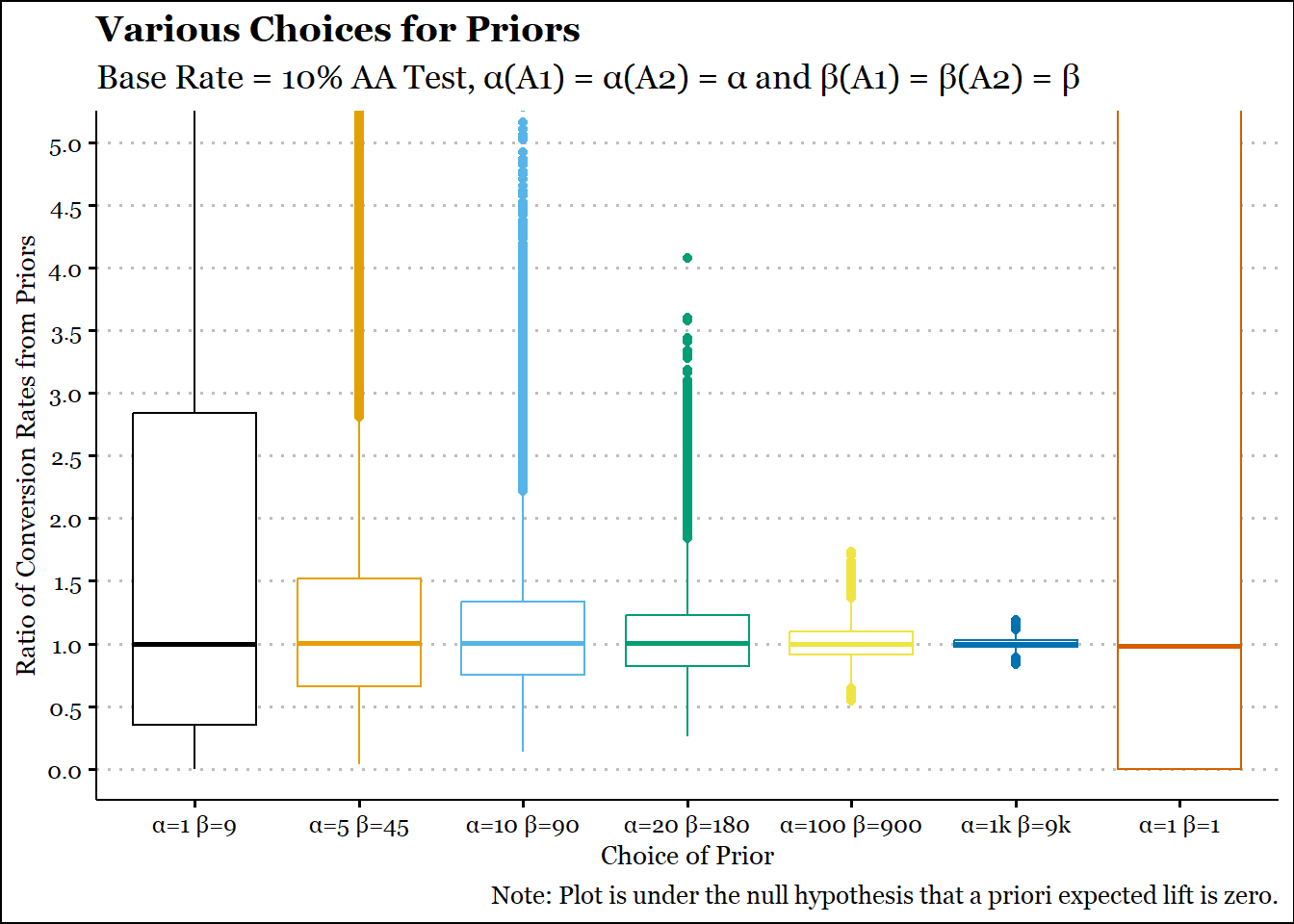
The key is defining a reasonable prior. There is no real point in using a Bayesian methodology if stronger assumptions aren’t made, so we won’t be using an uninformative prior like Beta(1,1). And since we are planning an A/A test, we will be keeping the parameters equal, i.e. 𝛂A1 = 𝛂A2 = 𝛂 and 𝛃A1 = 𝛃A2 = 𝛃.
We consider the historical rate of our design as 10%, so really, the question is whether the prior should be beta(10,90) or beta(1000,9000).
Show the code
p1 = .1q1 =1-p1prior_alpha =c(10,50,100,200,1000,10000,1)*p1prior_beta =c(10,50,100,200,1000,10000,1)*(1-p1)n_sim =10^5set.seed =145prior_ratios =pmap(list(.x = prior_alpha,.y = prior_beta, nn =n_sim),.f = \(.x,.y,nn) rbeta(nn,.x,.y)/rbeta(nn,.x,.y)) |>bind_cols() |>rename_with(.fn =~LETTERS[1:7]) |>pivot_longer(cols =everything(),names_to ='Priors',values_to ='Ratio') |>mutate(Priors =factor(Priors,ordered = T))ggplot(prior_ratios,aes(y = Ratio,x=Priors, col = Priors)) +geom_boxplot() +coord_cartesian(ylim =c(0, 5)) +labs(title ="Various Choices for Priors",subtitle ="Base Rate = 10% AA Test, \u03B1(A1) = \u03B1(A2) = \u03B1 and \u03B2(A1) = \u03B2(A2) = \u03B2",caption ="Note: Plot is under the null hypothesis that a priori expected lift is zero.",x ="Choice of Prior",y ="Ratio of Conversion Rates from Priors",parse = T) +scale_x_discrete(labels =paste0("\u03B1=",c("1","5","10","20","100","1k","1")," \u03B2=",c("9","45","90","180","900","9k","1"))) +scale_y_continuous(breaks =seq(0,5,.5), minor_breaks =seq(.25, 4.75,.5)) +scale_color_colorblind() +theme_clean() +theme(text=element_text(family="Georgia"), legend.position='none')
The choice of beta(10,90) seems reasonable. It doesn’t concentrate too heavily around a ratio of 1 and is more or less symmetric about 1. You can already see that the distributions can be right-skewed. Of course you could resolve that by using a difference instead of a ratio. But a ratio seems to be used more often by practitioners and proponents. The outcome of a beta(1,1) is also plotted for comparison. Clearly the range is too vast and it has no meaningful use.
Now let’s perform 10^4 A/A tests (lower count as we also need to simulate the posterior every time). But now comes the key question. In the frequentist paradigm, we just sampled from a normal distribution and each draw of \(\hat{p}\) was an A/A test.
In the Bayesian paradigm, we are dealing with the probability of an event. So, do we draw from the normal distribution or something else entirely? What we know is that the average rate has to be 10% and that we will collect some ‘n’ data-points. We can continue to keep the ‘n’ constant across all A/A tests. In fact, we had already assumed that our underlying data is binomially distributed - this is what allows our posterior to be beta distributed (read: conjugate priors).
We will use a nominal Type 1 Error Rae of 20%, a power of 90%, and an MDE of 5% to estimate the sample collected per A/A test per design. I understand that these are concepts from the frequentist paradigm, so we can say that we happen to collect the same amount of data and check if the rate of rejecting the null is similar – around 20%.
The table below indicates the number of times (% of simulations) we reject the null in favour of either A1 or A2:
Show the code
kable(dt1,digits =2,align ='c')
Table 1
Comparison
Nulls Rejected(%)
A2>A1
10.20
A1>A2
10.09
Our rate of rejecting the null was slightly higher than 20%.
This is despite the fact that using the same prior for both \(p_{A1}\) and \(p_{A2}\) should lower it as we are adding a priori evidence for the baseline being the same. In all honesty this is more or less a simulation artifact and we can use a stronger prior like beta(100,900). But the gaps in the beta-binomial approach should now be clear.
IBE Bayesian A/A Test - Conclusions
Notice how we consciously made a comparison on both sides (A2>A1 and A1>A2). When running an A/B test, we typically look to find evidence to justify a new design – there is a built-in directional bias. This gets reflected in the math when typically the ratio is compared on only one side. But an A/A test forces us to rethink this. Clearly the comparison should be made on both sides.
Before any data is collected, it is equally likely that design B is worse than design A. Yet, this isn’t taken into account when practitioners compare the ECDF of ratio of conversion rates solely in the direction where B is greater.
In practice, I have seen practitioners first check the direction, and then take the ratio as \(p_{b}/p_{a}\) or \(p_{a}/p_{b}\), whatever is convenient. It should be obvious that this is a post-hoc selection of direction, and obviously unless the p-value is halved, this is also equivalent to a 1-tailed test.
Once again, the problem isn’t the math, the problem is in the implementation. There are clear disadvantages to the IBE model.
A note on a weird prior selection method in the wild – The Time Series Trauma Technique
A primer about the beta distribution and its role as a prior
Here is a fun exercise: what does it really mean to say that your prior is beta(1,9)? In simple terms, it means that if you collected 10 data-points, one of them should indicate a conversion. The expected value of a beta distribution is usually \(\frac{\alpha}{\alpha+\beta}\), where \(\alpha\) and \(\beta\) are termed shape parameters. They essentially govern the shape of what the beta distribution would like on its support of 0 to 1. In essence, a beta distribution places weights on most likely conversion rates of an event.
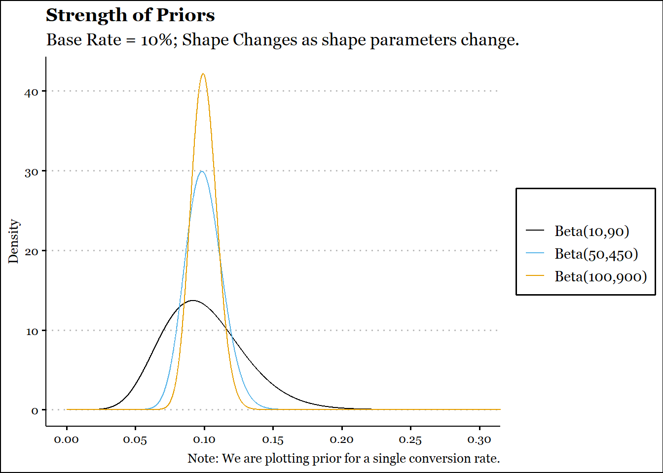
The expected value of beta(10,90) and beta(100,900) are the same, yet the latter is a much stronger assertion that the conversion rate is 10%. Think of it like drawing 100 data-points in the former case while drawing 1000 in the latter case, and then claiming that the observed conversion rate is 10%. The latter has a lower standard deviation and places more mass around 10% as opposed to the former.
Historical data can really only tell you about the former, and the choice of the shape parameters is essentially a choice in how strong you want your prior to be. This is the crux of the Bayesian Inference paradigm – choosing the appropriate strength of your prior once you have chosen the model.
Historical data isn’t going to help you in this regard. However, practical considerations force us to estimate how much data we reasonably expect to collect for an A/B test. If you have the luxury of being able to collect a lot of data for your A/B Test in a short span of time, then it doesn’t really matter whether you use a beta(1,1) model or a frequentist model or, heck, ask my mum to look at 10% and 12% after a million data points and see if she thinks B is better than A (spoiler alert: it’s always A; B is for those who didn’t work hard in school).
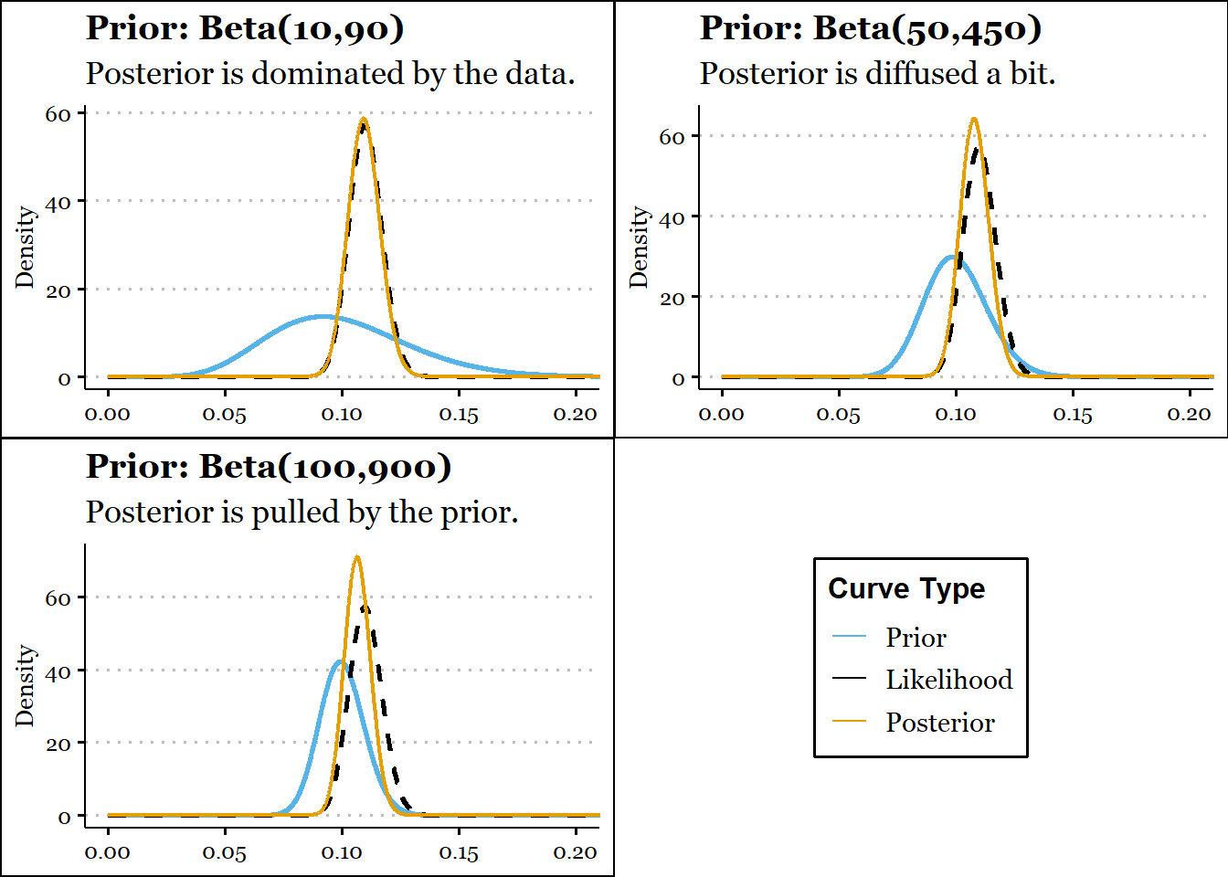
A reasonable rule of thumb can be – don’t make your prior dominate your data – unless you have good reasons for this to be the case. So, if you expect to collect 20K data-points per design, a prior like beta(10K,90K) can be highly inappropriate. You might as well not run the test, especially if the aim is to establish a decent magnitude of lift. Always remember:
The posterior distribution is a compromise between the prior and the likelihood as derived from the data.
Let’s try and see this from visualizations! We’ll plot a beta prior for a single conversion rate.
Show the code
p1 = .1q1 =1-p1chart_labs =c("Beta(10,90)","Beta(50,450)","Beta(100,900)")ggplot() +coord_cartesian(xlim =c(0,.3)) +geom_function(fun = dbeta, n =10^4, args=list(shape1=10,shape2=90), aes(col = chart_labs[1])) +geom_function(fun = dbeta, n =10^4, args=list(shape1=50,shape2=450), aes(col = chart_labs[2])) +geom_function(fun = dbeta, n =10^4, args=list(shape1=100,shape2=900), aes(col = chart_labs[3])) +guides(colour =guide_legend(title ="")) +labs(title ="Strength of Priors",subtitle ="Base Rate = 10%; Shape Changes as shape parameters change.",caption ="Note: We are plotting prior for a single conversion rate.",y ="Density",color ='Beta Priors',parse = T) +scale_x_continuous(breaks =seq(0,.3,.05), minor_breaks =seq(.025, .275,.05)) +scale_color_colorblind(breaks = chart_labs) +theme_clean() +theme(text=element_text(family="Georgia"),legend.text =element_text(family="Georgia"))
We can see above that as both α and β increase, the beta distribution gets narrower, i.e. the spread or standard deviation reduces. From the variance formula above we can see that the denominator grows faster than the numerator as either of those shape parameters increases.
Now let’s look at the impact of the prior on the posterior. To increase contrast, we’ll assume that the historical conversion rate was 10% for the design, but lately it’s been around 11%. We observe 2000 data-points. Note that we are still speaking of a single conversion rate in this illustrative example.
Using historical time-based data to estimate the shape parameters
Since we have two shape parameters, in order to estimate them from historical data, we’ll need two inputs. One is of course the average rate. If we can somehow insinuate a variance from somewhere, we’ll have a second parameter.
The variance of a conversion rate is generally expressed as \(\frac{p.(1-p)}{n}\), so if we were to keep aggregating data over a sufficiently large number of hours or days or weeks, our uncertainty in the conversion rate would be lowered, ceteris paribus (all else remaining equal, i.e., no structural shift in the conversion rate). Most often, we are talking about a conversion rate over the recent past, e.g., the most recent quarter.
Our variance input in this case is just a function of how much data we choose to aggregate, so to me at least this does not seem like a particularly useful method, but it can be made to work, when combined with an appropriate rule-of-thumb like the prior’s volume should not dominate that of the data you expect to collect.
A particularly diabolical approach that I have seen however is calculating the conversion rate over a fixed time-window for ‘T’ periods and then calculating the average and variance from there! Yes, you read that right, some people will calculate daily conversion rate over a 90-day period, then promptly use that to calculate a standard deviation. I cannot even begin to imagine how someone thought that calculating the standard deviation of the time series is the same as estimating the standard deviation of a conversion metric.
Then again, I have made my fair share of purgatorial choices, in life and in work. But let’s look at the impact of such a choice for building priors.
We’ll simulate a few conversion rate scenarios varying with some degree around 10%, and then we’ll calculate the average rate and standard deviation of the time-series over 30, 91 and 180 days.
Then we’ll reverse it and calculate the α and β parameters.
As the average daily conversion rate becomes more stable, the role of the prior becomes progressively larger. No surprises there. But what seems weird is that changing the number of days has a somewhat of an unpredictable impact. Sometimes it leads to a stronger prior while sometimes it leads to a weaker prior.
Again, this could very well be an artifact of simulation.
Nevertheless, I have great reservations about this approach for the following reason:
It says nothing about what is really going to happen with your experiment data. It could get drowned out by the prior, or it could make the prior completely redundant. Given that:
a Bayesian methodology is most often preferred where we expect to collect an insufficient amount of data w.r.t. a fixed-sample frequentist test of proportion,
We most often use the same prior for design A and B, which automatically means that the posterior lift is going to be less than the lift observed from raw data,
this style of building your prior is often going to drown your results exactly where you need support of modeled beliefs, especially on those assets where the conversion rate is more or less quite stable.
I am repeating myself here, but if you can collect a large amount of data for your experiment in a short span of time, Bayesian methodologies of any flavour aren’t going to give you a particularly contrary result as compared to the frequentist approach.
Crucially, this approach abstracts away the important practice, art and science of building principled priors, since your priors are essentially appearing auto-magically. We have also not talked about a scenario where there may be value in biasing your prior for a non-zero MDE (where you set α and β for the two designs distinctly) up front. While a rare situation, there are times when a non-zero null makes sense, either in a frequentist or a Bayesian approach.
…
We saw some pitfalls in how A/B tests based on IBE Bayesian approach can suffer from implementation errors and inadvertent inflation of Type 1 error rates.
We also a particularly weird way of defining priors.
Our final conclusion is that the problem is often between the chair and the keyboard, and in the fear of codifying your prior beliefs incorrectly, thereby screwing up your annual bonus.
In the next post we look at an alternative Bayesian methodology that potentially mitigates these implementation errors.